Filtering is used to make easier to focus on specific information on the large table of data. The records that will be displayed when filtered is the one who meets a certain criteria.
The data that aren’t meeting the criteria will be hidden and not deleted, so if you use a different criteria in your filter, the other data will be displayed.
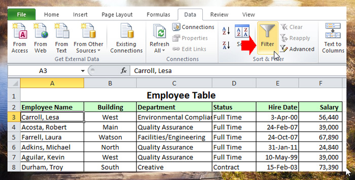
To add filtering in your worksheet table or database, click any cell inside the data set or table that you want to filter, then go to the Data Tab in the Ribbon, select “Filter” under Sort & Filter group.

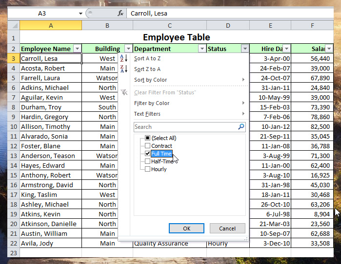
You will notice the table on the worksheet, will have an arrow-down in the column header, click the arrow on the column that you want to filter to reveal the drop-down menu. In the sample below I want only to display the full time employees, so I will select the full time in the status header filter menu and click ok to apply.

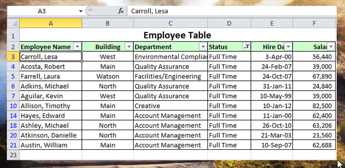
And this is the result after filtering.

To remove the filtering, click “Clear” in the data tab, if you want to remove all the filtering including the arrow-down menu in the header, click the Filter.

