Lookup functions in Excel are divided into two, VLookup (Vertical Lookup) function which look for the value in the leftmost column of the range of cells you specify in table-array and the HLookup (Horizontal Lookup) function look for value at the topmost row of the table array specified.
VLookup Function
VLookup function is used to find value from the leftmost column of the table-array and returns the value in the same row from different column you specify.
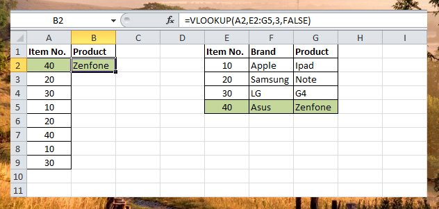
Take at look at the example below, VLookup function will search for the same value entered in A2, from the leftmost column in Table E2:G5, when vlookup finds exact match it will return the value from the same row from the third column which is set in the third argument.

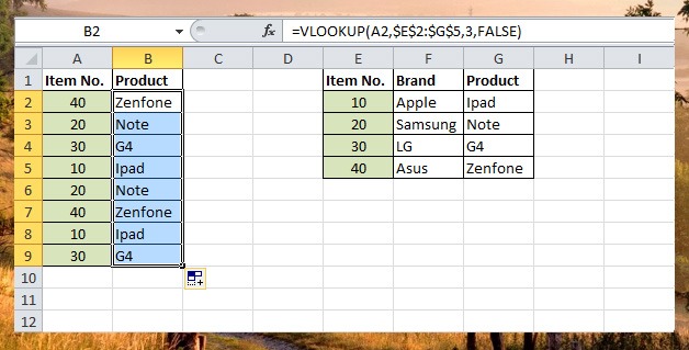
To make the Table E2:G5 absolute reference, we will add $ symbol before the Column letter and row number, so it will become $E$2:$G$5. Now that the reference table is fixed we can now drag the formula down from B2 to B9.

HLookup Function
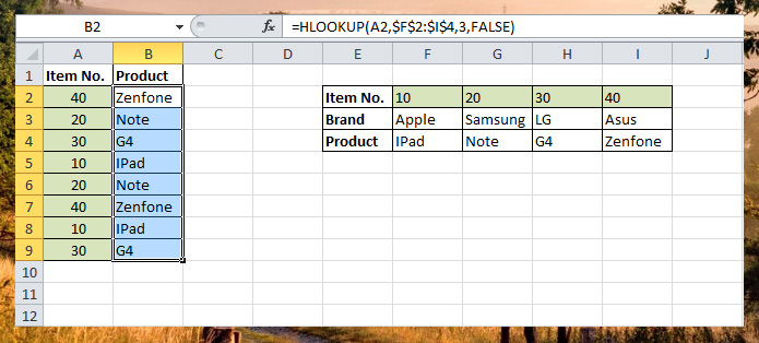
HLookup function work similar to vlookup but instead of searching for value from leftmost column it will search at the top row of the table-array.
We will revise the reference table we use in vlookup function to see the similarities.


what is the 3 and false int he formula
The number 3 in the VLookup formula is the 3rd column of the reference table which is the Product found in G column and in HLookup the 3rd row of the table which is also the product but in row 4.
The FALSE is a logical value that specifies whether you want VLOOKUP or HLOOKUP to find an exact match or an approximate match: This is optional, the formula will run without this.
TRUE assumes the first column in the table is sorted either numerically or alphabetically, and will then search for the closest value. This is the default method if you don’t specify one.
FALSE searches for the exact value in the first column.