Microsoft Excel is one of the most powerful tools for data analysis, and Conditional Formatting in Excel is an essential feature that enhances data visualization. It allows users to automatically format cells based on specific conditions, making it easier to identify trends, outliers, and important insights. Whether you’re working with financial data, reports, or spreadsheets, mastering conditional formatting can significantly improve your efficiency.
In this guide, we will explore:
- What conditional formatting is
- How to apply it in Excel
- Various types of conditional formatting rules
- Advanced techniques and best practices
What is Conditional Formatting in Excel?
Conditional Formatting in Excel is a feature that changes the appearance of a cell based on a specified condition or rule. You can apply different formats, such as font color, background color, or data bars, to highlight important data points.
This feature is useful for:
- Identifying duplicate values
- Highlighting values above or below a certain threshold
- Showing trends with color scales
- Visualizing data using icon sets
How to Apply Conditional Formatting in Excel
Applying conditional formatting in Excel is straightforward. Follow these steps to get started:
Step 1: Select the Data Range
- Open your Excel file and select the range of cells where you want to apply conditional formatting.
Step 2: Access the Conditional Formatting Menu
- Go to the Home tab.
- Click on Conditional Formatting in the ribbon.
Step 3: Choose a Formatting Rule
- Excel provides predefined rules such as Highlight Cells Rules, Top/Bottom Rules, Data Bars, Color Scales, and Icon Sets.
- Select a rule that fits your requirement.
Step 4: Customize the Rule
- If needed, you can enter specific values or criteria.
- Choose the formatting style (color, font, border, etc.).
Step 5: Apply the Rule
- Click OK to apply the conditional formatting.
- Your selected cells will now change their appearance based on the rule.
Types of Conditional Formatting Rules
1. Highlight Cells Rules
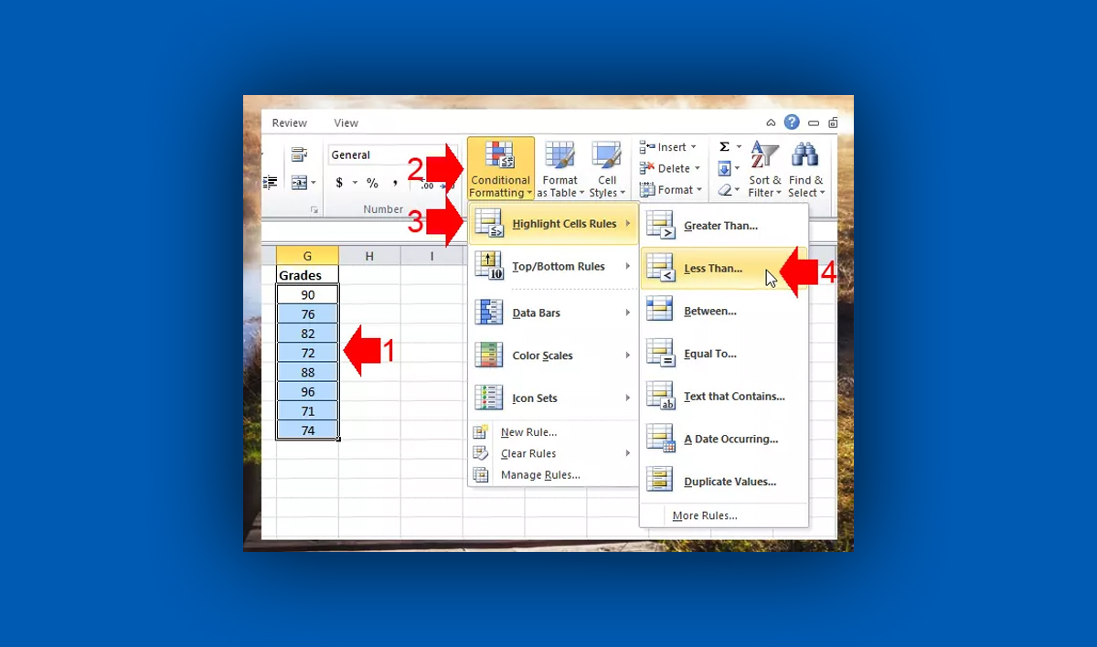
In the highlight cells rules, you can add formatting on the cells that contains greater than, less than, equal to, between, etc. In the example given below, we will highlight the cell that have failed grades. Follow the steps.
Step 1. Select the range of cells that you want to add formatting, on the Home tab, click Conditional Formatting, then on the drop-down select Highlight Cells Rules > Less than…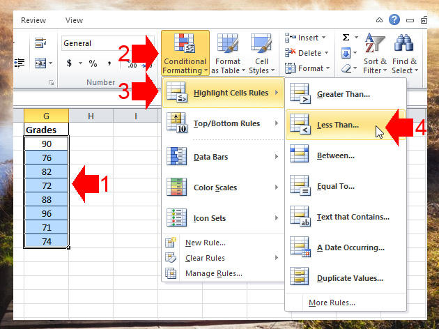
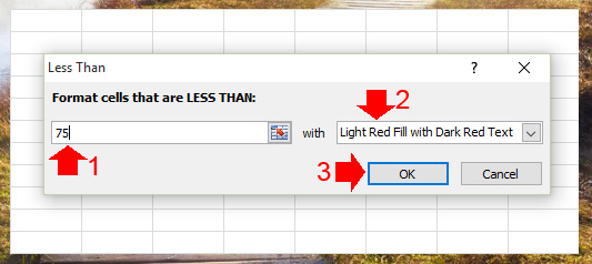
Step 2. Since we want to highlight the cells that are failed, we will enter the value 75. All the value less than 75 will be highlighted in red.
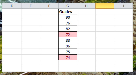
Step 3. This is the result after adding conditional formatting, everytime you enter less than 75 in the grades column it will be highlighted
You can use the same procedure in other conditional formatting rules, like greater than, top/bottom rules etc.
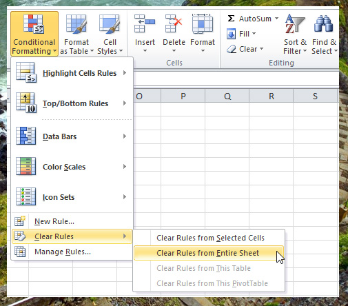
To clear the rules, go to Conditional Formatting in the Home tab, then select, Clear Rules on the drop-down, if you want to clear conditional formatting on the entire worksheet select “Clear Rules from Entire Sheet” or else select “Clear Rules from Selected Cells”.
2. Top/Bottom Rules
These rules help in identifying the highest and lowest values in a dataset.
- Top 10 items
- Top 10%
- Bottom 10 items
- Bottom 10%
- Above average / Below average
3. Data Bars
Data Bars provide a visual representation of data by filling cells with gradient or solid color bars. The length of the bar represents the value in the cell.
4. Color Scales
Color scales apply a gradient of colors based on the values in the selected range. For example:
- Green to red scale (high values are green, low values are red)
- Blue to white to red scale
5. Icon Sets
Excel provides icon sets that visually categorize data. Some common icon sets include:
- Traffic lights (red, yellow, green)
- Arrows (up, right, down)
- Shapes (circle, triangle, square)
Advanced Conditional Formatting Techniques
1. Using Formulas for Conditional Formatting
You can create custom rules using formulas. To do this:
- Go to Conditional Formatting > New Rule
- Select Use a formula to determine which cells to format
- Enter a formula (e.g.,
=A1>100to highlight values greater than 100) - Choose a format and click OK
2. Applying Conditional Formatting to Entire Rows
To highlight an entire row based on a condition in a specific column:
- Select the entire dataset.
- Use a formula like
=$B2="Completed"to highlight rows where column B contains “Completed”. - Apply a formatting style and confirm.
3. Combining Multiple Rules
You can apply multiple rules to the same range to enhance data visualization. For instance, you can use both Color Scales and Data Bars in the same range.
4. Managing and Removing Conditional Formatting
If you need to modify or remove conditional formatting:
- Select the formatted cells.
- Go to Conditional Formatting > Manage Rules.
- Edit or delete rules as needed.
Best Practices for Using Conditional Formatting in Excel
- Use Simple Rules: Avoid overcomplicating your spreadsheet with too many formatting rules, as it can become difficult to read.
- Optimize Performance: Conditional formatting can slow down large Excel files. Use it efficiently.
- Use Logical Colors: Choose colors that make sense (e.g., red for warnings, green for positive values).
- Test Before Applying to Large Datasets: Always test your formatting on a small range before applying it to an entire dataset.
- Document Formatting Rules: If you’re sharing your file, document what each rule does to avoid confusion.
Conclusion
Conditional Formatting in Excel is a powerful tool that enhances data analysis by making important information visually accessible. Whether you’re a beginner or an advanced Excel user, understanding how to apply and customize conditional formatting can greatly improve your efficiency and decision-making.
By following this guide, you can confidently apply conditional formatting to your spreadsheets and transform raw data into meaningful insights.
Check Also: Microsoft Excel 2021 Free Course