Conditional Formatting is used to highlight cells with certain value that meet the condition set. There are several condition rules that you can use to format your worksheet like highlight cells rules, Top/Bottom Rules, etc.
For example, when making class records, to easily see the failed students, you can easily add formatting on the grades that is below the average.
Highlight Cells Rules
In the highlight cells rules, you can add formatting on the cells that contains greater than, less than, equal to, between, etc. In the example given below, we will highlight the cell that have failed grades. Follow the steps.
Step 1. Select the range of cells that you want to add formatting, on the Home tab, click Conditional Formatting, then on the drop-down select Highlight Cells Rules > Less than…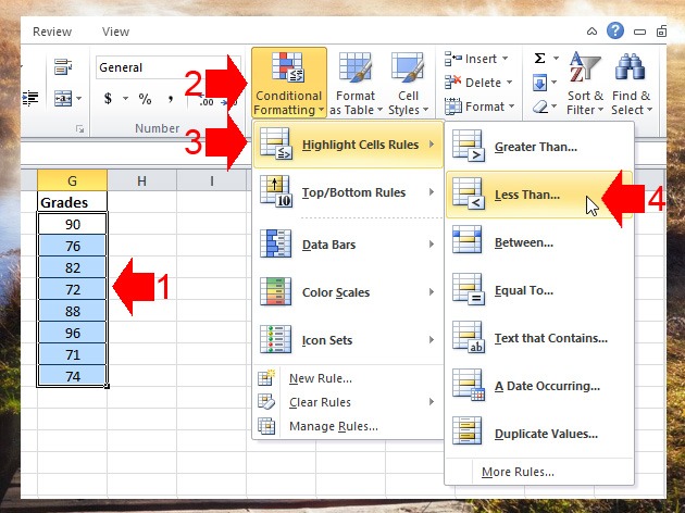
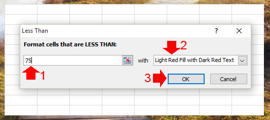
Step 2. Since we want to highlight the cells that are failed, we will enter the value 75. All the value less than 75 will be highlighted in red.
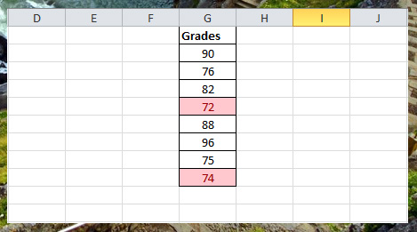
Step 3. This is the result after adding conditional formatting, everytime you enter less than 75 in the grades column it will be highlighted
You can use the same procedure in other conditional formatting rules, like greater than, top/bottom rules etc.
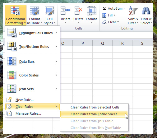
To clear the rules, go to Conditional Formatting in the Home tab, then select, Clear Rules on the drop-down, if you want to clear conditional formatting on the entire worksheet select “Clear Rules from Entire Sheet” or else select “Clear Rules from Selected Cells”.